| MATLAB:
Solution of Linear Systems of Equations |
| As you read this material we strongly recommend that you activate your MATLAB window and try the commands explained right there and then. |
There are many various ways of solving linear systems of equations.Ā We can classify them as:
1) Direct methods
In this category we can list the various row reduction algorithms available.Ā Most of these algorithms can be easily programmed in a basic programming language such as C++.Ā They can also be programmed in MATLAB and there are various software libraries, which contain superb programs and functions for the solution of linear systems.
In order to have an idea about these methods we will go over a very simple example using the upper triangularization technique.
Consider the system A x = B withĀ
 ĀĀ
ĀĀ
as a first step we form the ōaugmented matrixö by placing B as the fourth column of A.Ā We then proceed to add ( or subtract) appropriate multiples of the first equation from the other two so that the numbers in locationsĀ 2,1 and 3,1 of the matrix become zero.Ā We should only remember the basic properties of equality, to convince ourselves that this type of algebraic manipulation does not alter the roots of the system.Ā In other words, the system obtained after these row operations has the same roots as the original system, as we say, it is equivalent.Ā We proceed with the row reduction until the coefficient matrix becomes triangular .
We can now solve the system easily by performing a backward substitution.Ā What we mean is this: first solve the last equation for x3 to obtain
x3 = 3 / 7,
then use the second equation to obtain x2 as
x2 = (2 / 7) * ( 3 / 2 Ł (-7 / 2 ) * x3) = 6 / 7,
and finally use the first equation to obtain x1 as
x1 = (1 / 2) * ( 1 Ł (-1) * x2 Ł 3 * x3 = 2 / 7.
The corner elements of the upper triangular matrix ( the ones on the diagonal) are called pivot elements.Ā The larger the absolute value of these elements , relative to the other elements of the row, the more stable the solution is.Ā Some solution methods exchange the order of equations in order to achieve the maximum pivot elements.Ā Pivoting is actually strongly recommended for any serious program designed for the solution of linear systems of equations.
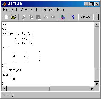
For completeness we should mention CramerÆs Rule , which utilizes determinants for the solution of systems. Determinant is a number associated with a square matrix.Ā We will not learn here how to calculate determinants by hand, but MATLAB gives the determinant of a matrix by the use of the commandĀ det(a).Ā See the example below:
CramerÆs rule produces the solution of a system A x = B as follows: ĀĀĀĀĀĀĀĀĀĀĀĀĀ ĀĀĀĀĀ
| The first unknown is given byĀ |
x1 = det( A1 ) / det( A ) |
| The second by |
x2 = det( A2 ) / det( A ), |
| The third by |
x3 = det( A3 ) / det( A ), |
And so onģ.Ā Here A1 is the matrix obtained by replacing the first column of A by B, A2 is the matrix obtained by replacing the second column of A by B etcģ.Ā It is easy to see that if det( A ) is zero or close to zero we get into trouble.Ā Well posed engineering problems avoid this type of ōill conditioningö .
2) Iterative methods
There are various methods in this category.Ā The general idea is that we start with an arbitrary guess for the solution and then we use the equations to progressively improve the solution ( very much like NewtonÆs method).Ā The most popular and in fact easy method is the Gauss Siedel method of iteration.Ā Here each equation is solved for one of the unknowns in terms of the remaining ones, then using the initial guess a new solution is obtained which is , in turn, substituted into the equations to yield an improved estimate and so on..Ā We give an example below:
Consider again the system A x = B withĀ
 ĀĀ
.
ĀĀ
.
We write:
x1 = ( 1 + x2 Ł 3 * x3) / 2 ģģ.. eq. 1
x2 = ( 2 Ł x1 + 2 * x3 ) / 3Ā ģģ.eq. 2
x3 = ( 3 Ł 3 * x1 ) / 5Ā ģģģģ.eq. 3
Now we start with the initial guessĀ [0, 0, 0] and using equationĀ (1) we obtain [ 0.5, 0, 0] .Ā Using this in equation (2) we obtain [ 0.5, 0.5, 0] and using this in equation (3) we obtainĀ [0.5, 0.5, 0.3].Ā We now go back to equation (1) and obtain [0.3, 0.5, 0.3]Ā repeating this cycle produces the approximations shown ( obtained using excel):
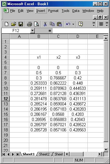
We can check and see that the unknowns converged well ( four significant digits)Ā to the ōexactö values:Ā [ 2 / 7, 6 / 7, 3 / 7 ] .
3)Ā Piece of cake methods
Here we use a package to obtain the solution of the system.Ā This package may be MAPLE, it could be Excel, but the ideal one is MATLAB.
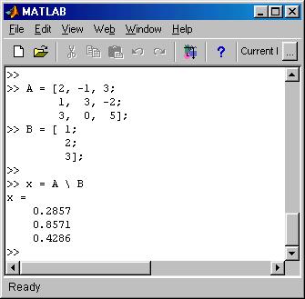
The command for solving the systemĀ AĀ x = B is simplyĀĀ x = A \ B.Ā The following picture demonstrates this:
The inverse of a matrix:
A special square matrix is the ōidentityö matrix.Ā This matrix has 1Æs seating on each place of its main diagonal, and zero everywhere else.Ā For example the 3X3 identity matrix is:

Now we can pose the following problem:ö If a nXnĀ square matrix A is known, can we find a matrix A-1 so that
A A-1 = identity matrix.
The matrix A-1 is called the inverse of A.Ā If you think carefully you will see that the columns of the inverse are obtained by solving n systems of equations which have the form
A x = d
With d being the individual columns of the identity matrix.
Thinking again carefully you will see that the solution of a system of equationsĀ
A x = B ,
c an be formally written as:
x = A-1 B
( this is the sequence:)
A x = B
A-1 A x = A-1 B
IdentityĀ x = A-1 B
x = A-1 B
Of course MATLAB calculates the inverse with extreme ease.
The following picture demonstrates this approach in solving the example system:
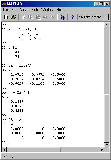
Note that the last operation is only a check on the calculations of the inverse of matrix A.Ā The minus zeros that appear in three places are small in absolute value numbers which show up due to round off error.