| MATLAB:
Linear Systems of Equations - Matrix Multiplication |
| As you read this material we strongly recommend that you activate your MATLAB window and try the commands explained right there and then. |
A great number of engineering problems require the solution of a system of linear equations.Ā These systems may consist of 3 Ł 4 equations or may be comprised of hundreds of equations.Ā We have all seen some linear systems in arithmetic, high school algebra and pre calculus courses.Ā A four by four system looks like this:
a11 x1 + a12 x2 + a13 x3 + a14 x4 = b1
a21 x1 + a22 x2 + a23 x3 + a24 x4 = b2
a31 x1 + a32 x2 + a33 x3 + a34 x4 = b3
a41 x1 + a42 x2 + a43 x3 + a44 x4 = b4
Here the aÆs and the bÆs are known numbers and the xÆs are the unknowns to be determined by the solution of the system.Ā The reason these equations are called ōlinearö is that the unknowns appear only in the first power: no square, no powers, no transcendental functions Ālike sin (x2) or e x1.
The following table gives a few examples of engineering problems that require the solution of linear systems.
| Some engineering problems which require the solution of linear systems of equations |
|
|
Goal:Ā To determine the forces acting on elements of trusses and frames Principle used:Ā Balance of forces at each node (points where the elements meet) |
|
|
Goal:Ā To determine the equilibrium temperature distribution in a metal plate with one side much hotter than the others.Principle used:Ā Heat balance equations are written in discrete form using finite difference approximation. |
|
|
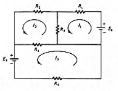
Goal:Ā To determine the electric current in each segment of the circuit Principle used: KirchhoffÆs Ājunction rule (it reduces the number of unknown currents to three )Ā and loop rule ( produces three equations for the currentsĀ I1, I2 and I3) . |
| Ā
|
Goal:Ā Characterization of residual stresses in Functionally Graded Materials (FGM) Principle used:Ā Equations of elasticity are written in discrete form using Finite Elements Modeling (FEM). Experiments evaluate the accuracy of modeling.
|
| Ā
|
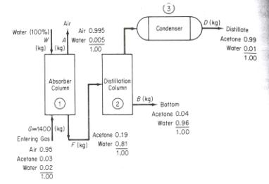
Goal: Given the flow rate of the entering gas, to determine the flow rate of the distillate acetone ( as well as the other Āflow rates ). Principle used: Material balance equations are written for the absorber column, the distillation column and for the condenser. ( more complex problems involve chemical reactions) |
| Ā
|
A product optimization problem Goal: Mixing quantities of the available foods to synthesize the ōideal foodö at minimum cost. Principle used: The matrix of nutrient content is known. The nutrient requirements of an ideal diet are given as a mX1 array.Ā The unit cost of each food is also known. |
Writing a system in terms of arrays.
When we look at the system given at the top of this file, it is evident that the xÆs are needlessly repeated in each line of the system. It makes a lot of sense to develop some sort of notation, which will eliminate the need to write them again and again in each of the equations.Ā This notation is supplied by the introduction of a new array operation known as matrix multiplication.
Let us first consider a simple example:
We have a 3X4 matrix AĀ and a 4X1 matrix B defined as:
Ā
 Ā.
Ā.
The product of the two matrices , noted as AB is another matrix C having 3 rows and 1 column.Ā The elements of this matrix C are obtained by adding the products of the numbers in the rows of A with the numbers in the column of matrix B.Ā This is what we get:
As we can see, for this definition to make sense, the number of columns of the first matrix must match the number of rows of the second matrix. It also implies that the resulting matrix C will have the same number of rows as the first matrix and the same number of columns as the second matrix i.e.
( M X N ) ( N X K ) Ó ( M X K )
When the second matrix has more than one columns, then we multiply each of its columns with the first matrix as shown above for the single column.
This is a more general example:
Of course,Ā MATLAB is very good at matrix multiplication. All we have to do is define the arrays and then write A * B.Ā Here is the above example worked by MATLAB:

In order to write our linear system of equations in matrix notation, we need one more concept.Ā This is the concept of equality of matrices.
When we write A = B and a, b are matrices we imply the following:
1) both matrices have the same number of rows and the same number of columns
2) each and every element of matrix A is equal to the corresponding element of the matrix B.
Example:
![]() ĀĀ implies that a = 3, b = 5, c
= 1, and d = 7.
ĀĀ implies that a = 3, b = 5, c
= 1, and d = 7.
We are now ready to write our system in matrix form, we write
A x = B
WhereĀĀĀ
ĀNote that matrix names are usually written with bold face letters or with an ~ underline.